brinla
INLA Split Plot Model example
Julian Faraway 22 September 2020
See the introduction for an overview. Load the libraries:
library(ggplot2)
library(INLA)
Data
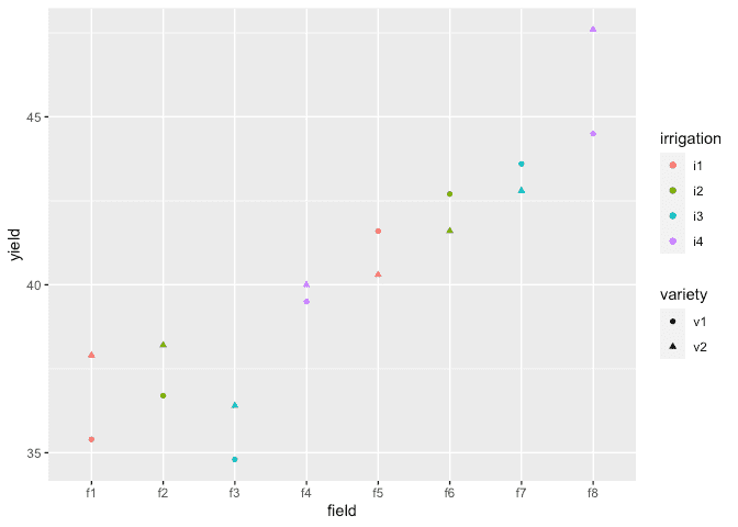
Load in and plot the data:
data(irrigation, package="faraway")
summary(irrigation)
     field   irrigation variety     yield
 f1     :2   i1:4       v1:8    Min.   :34.8
 f2     :2   i2:4       v2:8    1st Qu.:37.6
 f3     :2   i3:4               Median :40.1
 f4     :2   i4:4               Mean   :40.2
 f5     :2                      3rd Qu.:42.7
 f6     :2                      Max.   :47.6
 (Other):4
ggplot(irrigation, aes(y=yield, x=field, shape=variety, color=irrigation)) + geom_point()
Default INLA fit
formula <- yield ~ irrigation + variety +f(field, model="iid")
result <- inla(formula, family="gaussian", data=irrigation)
result <- inla.hyperpar(result)
summary(result)
Call:
   "inla(formula = formula, family = \"gaussian\", data = irrigation)"
Time used:
    Pre = 1.34, Running = 0.141, Post = 0.0792, Total = 1.56
Fixed effects:
               mean    sd 0.025quant 0.5quant 0.975quant   mode kld
(Intercept)  38.469 2.810     32.829   38.461     44.151 38.452   0
irrigationi2  0.949 3.949     -7.047    0.957      8.876  0.969   0
irrigationi3  0.552 3.949     -7.442    0.560      8.481  0.571   0
irrigationi4  4.024 3.949     -3.986    4.037     11.939  4.054   0
varietyv2     0.750 0.618     -0.491    0.750      1.989  0.750   0

Random effects:
  Name    Model
    field IID model

Model hyperparameters:
                                         mean    sd 0.025quant 0.5quant 0.975quant  mode
Precision for the Gaussian observations 0.867 0.428      0.224    0.802      1.875 0.672
Precision for field                     0.105 0.076      0.020    0.088      0.288 0.061

Expected number of effective parameters(stdev): 8.71(0.29)
Number of equivalent replicates : 1.84

Marginal log-Likelihood:  -66.93
Default looks more plausible than one way and RBD examples.
Compute the transforms to an SD scale for the field and error. Make a table of summary statistics for the posteriors:
sigmaalpha <- inla.tmarginal(function(x) 1/sqrt(exp(x)),result$internal.marginals.hyperpar[[2]])
sigmaepsilon <- inla.tmarginal(function(x) 1/sqrt(exp(x)),result$internal.marginals.hyperpar[[1]])
restab=sapply(result$marginals.fixed, function(x) inla.zmarginal(x,silent=TRUE))
restab=cbind(restab, inla.zmarginal(sigmaalpha,silent=TRUE))
restab=cbind(restab, inla.zmarginal(sigmaepsilon,silent=TRUE))
colnames(restab) = c("mu","ir2","ir3","ir4","v2","alpha","epsilon")
data.frame(restab)
               mu     ir2     ir3     ir4       v2  alpha epsilon
mean       38.469 0.94858 0.55178  4.0238  0.74971 3.6514   1.191
sd         2.8106  3.9501  3.9501  3.9503  0.61835 1.3537  0.3602
quant0.025 32.823 -7.0565 -7.4515 -3.9959 -0.49254 1.8567 0.73092
quant0.25  36.772 -1.4166 -1.8137  1.6614  0.36647 2.7362 0.94892
quant0.5   38.447 0.93806 0.54067  4.0178  0.74668 3.3724  1.1156
quant0.75  40.129  3.2859  2.8887   6.364   1.1269 4.2396  1.3409
quant0.975 44.136  8.8579  8.4629  11.919   1.9856 7.0837  2.1047
Also construct a plot the SD posteriors:
ddf <- data.frame(rbind(sigmaalpha,sigmaepsilon),errterm=gl(2,nrow(sigmaalpha),labels = c("alpha","epsilon")))
ggplot(ddf, aes(x,y, linetype=errterm))+geom_line()+xlab("yield")+ylab("density")+xlim(0,10)
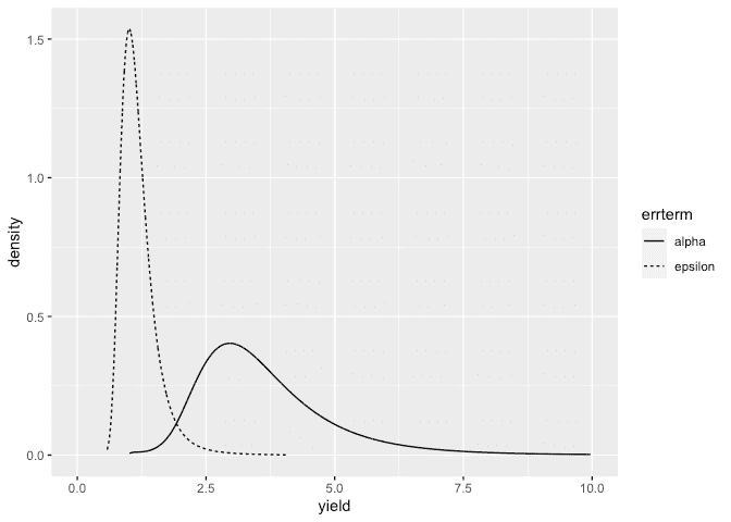
Posteriors look OK.
Informative Gamma priors on the precisions
Now try more informative gamma priors for the precisions. Define it so
the mean value of gamma prior is set to the inverse of the variance of
the residuals of the fixed-effects only model. We expect the two error
variances to be lower than this variance so this is an overestimate. The
variance of the gamma prior (for the precision) is controlled by the
apar shape parameter.
apar <- 0.5
lmod <- lm(yield ~ irrigation+variety, data=irrigation)
bpar <- apar*var(residuals(lmod))
lgprior <- list(prec = list(prior="loggamma", param = c(apar,bpar)))
formula = yield ~ irrigation+variety+f(field, model="iid", hyper = lgprior)
result <- inla(formula, family="gaussian", data=irrigation)
result <- inla.hyperpar(result)
summary(result)
Call:
   "inla(formula = formula, family = \"gaussian\", data = irrigation)"
Time used:
    Pre = 1.32, Running = 0.153, Post = 0.0842, Total = 1.56
Fixed effects:
               mean    sd 0.025quant 0.5quant 0.975quant   mode kld
(Intercept)  38.491 3.440     31.569   38.477     45.489 38.462   0
irrigationi2  0.924 4.844     -8.936    0.939     10.674  0.958   0
irrigationi3  0.529 4.844     -9.328    0.542     10.281  0.560   0
irrigationi4  3.986 4.845     -5.899    4.009     13.713  4.037   0
varietyv2     0.750 0.605     -0.463    0.750      1.961  0.750   0

Random effects:
  Name    Model
    field IID model

Model hyperparameters:
                                         mean    sd 0.025quant 0.5quant 0.975quant  mode
Precision for the Gaussian observations 0.892 0.425      0.260    0.826      1.896 0.692
Precision for field                     0.070 0.047      0.012    0.059      0.188 0.039

Expected number of effective parameters(stdev): 8.80(0.193)
Number of equivalent replicates : 1.82

Marginal log-Likelihood:  -55.86
Compute the summaries as before:
sigmaalpha <- inla.tmarginal(function(x) 1/sqrt(exp(x)),result$internal.marginals.hyperpar[[2]])
sigmaepsilon <- inla.tmarginal(function(x) 1/sqrt(exp(x)),result$internal.marginals.hyperpar[[1]])
restab=sapply(result$marginals.fixed, function(x) inla.zmarginal(x,silent=TRUE))
restab=cbind(restab, inla.zmarginal(sigmaalpha,silent=TRUE))
restab=cbind(restab, inla.zmarginal(sigmaepsilon,silent=TRUE))
colnames(restab) = c("mu","ir2","ir3","ir4","v2","alpha","epsilon")
data.frame(restab)
               mu     ir2     ir3     ir4       v2  alpha epsilon
mean       38.491 0.92369 0.52856  3.9859  0.74973 4.5237  1.1611
sd         3.4413  4.8459  4.8459  4.8464  0.60482 1.8183 0.31715
quant0.025 31.561 -8.9479 -9.3396 -5.9123 -0.46439 2.3073 0.72703
quant0.25  36.456 -1.9131 -2.3089   1.154   0.3723 3.3008 0.93973
quant0.5    38.46 0.91484 0.51868  3.9851  0.74676 4.1029  1.0997
quant0.75  40.474  3.7313  3.3355  6.7988   1.1212 5.2456  1.3111
quant0.975 45.469   10.65  10.258  13.688   1.9576 9.2349  1.9532
Make the plots:
ddf <- data.frame(rbind(sigmaalpha,sigmaepsilon),errterm=gl(2,nrow(sigmaalpha),labels = c("alpha","epsilon")))
ggplot(ddf, aes(x,y, linetype=errterm))+geom_line()+xlab("yield")+ylab("density")+xlim(0,10)
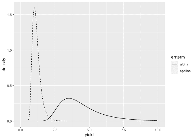
Posteriors look OK.
Penalized Complexity Prior
In Simpson et al (2015), penalized complexity priors are proposed. This requires that we specify a scaling for the SDs of the random effects. We use the SD of the residuals of the fixed effects only model (what might be called the base model in the paper) to provide this scaling.
lmod <- lm(yield ~ irrigation+variety, irrigation)
sdres <- sd(residuals(lmod))
pcprior <- list(prec = list(prior="pc.prec", param = c(3*sdres,0.01)))
formula <- yield ~ irrigation+variety+f(field, model="iid", hyper = pcprior)
result <- inla(formula, family="gaussian", data=irrigation)
result <- inla.hyperpar(result)
summary(result)
Call:
   "inla(formula = formula, family = \"gaussian\", data = irrigation)"
Time used:
    Pre = 1.32, Running = 0.145, Post = 0.0828, Total = 1.55
Fixed effects:
               mean    sd 0.025quant 0.5quant 0.975quant   mode kld
(Intercept)  38.477 3.042     32.361   38.469     44.639 38.457   0
irrigationi2  0.940 4.280     -7.731    0.949      9.549  0.962   0
irrigationi3  0.544 4.280     -8.125    0.552      9.154  0.565   0
irrigationi4  4.011 4.281     -4.674    4.025     12.604  4.045   0
varietyv2     0.750 0.606     -0.467    0.750      1.964  0.750   0

Random effects:
  Name    Model
    field IID model

Model hyperparameters:
                                         mean    sd 0.025quant 0.5quant 0.975quant  mode
Precision for the Gaussian observations 0.886 0.425      0.253     0.82      1.891 0.686
Precision for field                     0.082 0.053      0.018     0.07      0.214 0.049

Expected number of effective parameters(stdev): 8.77(0.215)
Number of equivalent replicates : 1.82

Marginal log-Likelihood:  -56.40
Compute the summaries as before:
sigmaalpha <- inla.tmarginal(function(x) 1/sqrt(exp(x)),result$internal.marginals.hyperpar[[2]])
sigmaepsilon <- inla.tmarginal(function(x) 1/sqrt(exp(x)),result$internal.marginals.hyperpar[[1]])
restab=sapply(result$marginals.fixed, function(x) inla.zmarginal(x,silent=TRUE))
restab=cbind(restab, inla.zmarginal(sigmaalpha,silent=TRUE))
restab=cbind(restab, inla.zmarginal(sigmaepsilon,silent=TRUE))
colnames(restab) = c("mu","ir2","ir3","ir4","v2","alpha","epsilon")
data.frame(restab)
               mu     ir2     ir3     ir4       v2  alpha epsilon
mean       38.477 0.93976 0.54353  4.0106  0.74972 4.0372  1.1676
sd         3.0424  4.2806  4.2806  4.2808  0.60614 1.3393 0.32498
quant0.025 32.355 -7.7417 -8.1361 -4.6858 -0.46761 2.1601 0.72807
quant0.25  36.614 -1.6624  -2.059  1.4111  0.37106 3.0892 0.94212
quant0.5   38.454 0.92811 0.53126  4.0037  0.74674 3.7841  1.1037
quant0.75    40.3  3.5109  3.1143  6.5847   1.1224 4.7019  1.3181
quant0.975 44.617  9.5218  9.1274  12.579   1.9608 7.3651  1.9816
Make the plots:
ddf <- data.frame(rbind(sigmaalpha,sigmaepsilon),errterm=gl(2,nrow(sigmaalpha),labels = c("alpha","epsilon")))
ggplot(ddf, aes(x,y, linetype=errterm))+geom_line()+xlab("yield")+ylab("density")+xlim(0,10)
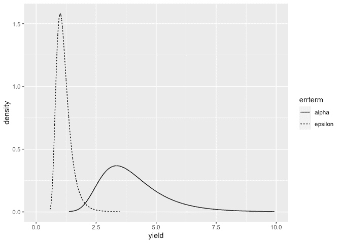
Posteriors look OK.
Package version info
sessionInfo()
R version 4.0.2 (2020-06-22)
Platform: x86_64-apple-darwin17.0 (64-bit)
Running under: macOS Catalina 10.15.6

Matrix products: default
BLAS:   /Library/Frameworks/R.framework/Versions/4.0/Resources/lib/libRblas.dylib
LAPACK: /Library/Frameworks/R.framework/Versions/4.0/Resources/lib/libRlapack.dylib

locale:
[1] en_GB.UTF-8/en_GB.UTF-8/en_GB.UTF-8/C/en_GB.UTF-8/en_GB.UTF-8

attached base packages:
[1] parallel  stats     graphics  grDevices utils     datasets  methods   base

other attached packages:
[1] INLA_20.03.17 foreach_1.5.0 sp_1.4-2      Matrix_1.2-18 ggplot2_3.3.2 knitr_1.29

loaded via a namespace (and not attached):
 [1] pillar_1.4.6         compiler_4.0.2       iterators_1.0.12     tools_4.0.2          digest_0.6.25
 [6] evaluate_0.14        lifecycle_0.2.0      tibble_3.0.3         gtable_0.3.0         lattice_0.20-41
[11] pkgconfig_2.0.3      rlang_0.4.7          yaml_2.2.1           xfun_0.16            withr_2.2.0
[16] dplyr_1.0.2          stringr_1.4.0        MatrixModels_0.4-1   generics_0.0.2       vctrs_0.3.4
[21] grid_4.0.2           tidyselect_1.1.0     glue_1.4.2           R6_2.4.1             rmarkdown_2.3
[26] farver_2.0.3         purrr_0.3.4          magrittr_1.5         splines_4.0.2        scales_1.1.1
[31] codetools_0.2-16     ellipsis_0.3.1       htmltools_0.5.0.9000 colorspace_1.4-1     Deriv_4.0.1
[36] labeling_0.3         stringi_1.4.6        munsell_0.5.0        crayon_1.3.4