brinla
Confidence bands for smoothness with Gaussian process regression using INLA ================ Julian Faraway 21 February 2022
See the introduction for more about INLA. See an example of Gaussian process regression using the same data. The construction is detailed in our book.
Load the packages (you may need to install the brinla package)
library(INLA)
library(brinla)
Data
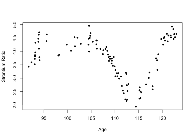
We use the fossil example from (Bralower et al. 1997) and used by (Chaudhuri and Marron 1999). We have the ratio of strontium isotopes found in fossil shells in the mid-Cretaceous period from about 90 to 125 million years ago. We rescale the response as in the SiZer paper.
data(fossil, package="brinla")
fossil$sr <- (fossil$sr-0.7)*100
Plot the data:
plot(sr ~ age, fossil, xlab="Age",ylab="Strontium Ratio")
GP fitting
The default fit uses priors based on the SD of the response and the range of the predictor to motivate sensible priors.
gpmod = bri.gpr(fossil$age, fossil$sr)
We can plot the resulting fit and 95% credible bands
plot(sr ~ age, fossil, xlab="Age",ylab="Strontium Ratio")
lines(gpmod$xout, gpmod$mean)
lines(gpmod$xout, gpmod$lcb, lty=2)
lines(gpmod$xout, gpmod$ucb, lty=2)
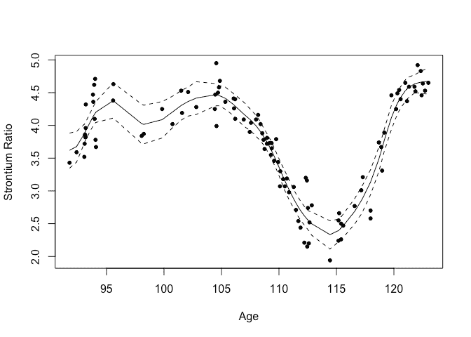
What do these bands represent? At any given value of the predictor (in this case, the age), we have a posterior distribution for the strontium ratio. The credible interval at this value of age is computed from the the 2.5% and 97.5% percentiles of this distribution. It expresses the uncertainty about the response at this predictor value.
Confidence bands for smoothness
The bands are constructed from joining all the pointwise intervals. This gives us a sense of the uncertainty of the response curve. But the value of these bands is limited. We might wish to say that curves falling within these bands have high probability while those that venture outside have lower probability. But this would not be entirely true. The bands tells us little about how rough or smooth the curve is likely to be. A rough sawtooth function could fit between the bands but is it plausible?.
In (Chaudhuri and Marron 1999), the question of whether there really is a dip (local minimum) in the response around 98 million years ago is asked. Notice that we could easily draw a function between the upper and lower bands that has no dip in this region. In contrast, we are sure there is a dip at 115 million years as the bands are tight enough to be clear about this. So do we conclude there is no strong evidence of a dip at 98?
The presence of a dip at 98 is strongly determined by how much we smooth the function. Gaussian process regression controls this primarily through the range parameter. The curves shown on the figure derive from the maximum posterior value of this parameter. Yet there is considerable uncertainty in this parameter which has its own posterior distribution. We take the 2.5% and 97.5% percentiles of this range posterior and then plot the resulting function with the other parameters set at their maximum posterior values. The resulting two curves are shown in the following figure:
fg <- bri.smoothband(fossil$age, fossil$sr)
plot(sr ~ age, fossil)
lines(fg$xout, fg$rcb,lty=1)
lines(fg$xout, fg$scb,lty=2)
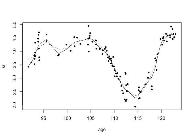
The solid line is lower band for the range parameter representing the rougher end of the fit. The dashed line is the upper band for the range parameter representing the smoother end of the fit. Both curves show a dip at 98 (although the dip is very shallow for the smoother curve). Thus we conclude there is a good evidence of a dip at 98. We can also see that the amount of smoothing has very little impact on the shape of the curve for the right end of the curve. In contrast, it makes a big difference on the left end of the curve.
I argue that these bands are often more useful in expressing the uncertainty in a fit than the usual bands. We are often more interested in the shape of the fitted curve than its specific horizontal level. Here is some more discussion about the deficiencies of standard confidence bands and confidence bands for smoothness. I have also have a paper, (Faraway 2016) on the topic.
Package versions
sessionInfo()
R version 4.1.0 (2021-05-18)
Platform: x86_64-apple-darwin17.0 (64-bit)
Running under: macOS Big Sur 10.16

Matrix products: default
BLAS:   /Library/Frameworks/R.framework/Versions/4.1/Resources/lib/libRblas.dylib
LAPACK: /Library/Frameworks/R.framework/Versions/4.1/Resources/lib/libRlapack.dylib

locale:
[1] en_GB.UTF-8/en_GB.UTF-8/en_GB.UTF-8/C/en_GB.UTF-8/en_GB.UTF-8

attached base packages:
[1] parallel  stats     graphics  grDevices utils     datasets  methods   base

other attached packages:
[1] brinla_0.1.0  INLA_22.01.25 sp_1.4-6      foreach_1.5.2 Matrix_1.4-0  knitr_1.37

loaded via a namespace (and not attached):
 [1] rstudioapi_0.13    magrittr_2.0.2     splines_4.1.0      lattice_0.20-45    Deriv_4.1.3        rlang_1.0.1
 [7] fastmap_1.1.0      stringr_1.4.0      highr_0.9          tools_4.1.0        grid_4.1.0         xfun_0.29
[13] cli_3.1.1          htmltools_0.5.2    iterators_1.0.14   MatrixModels_0.5-0 yaml_2.2.2         digest_0.6.29
[19] codetools_0.2-18   evaluate_0.14      rmarkdown_2.11     stringi_1.7.6      compiler_4.1.0