brinla
One way ANOVA - reeds
Julian Faraway 21 September 2020
See the introduction for an overview. Load the libraries:
library(ggplot2)
library(INLA)
library(brinla)
Data
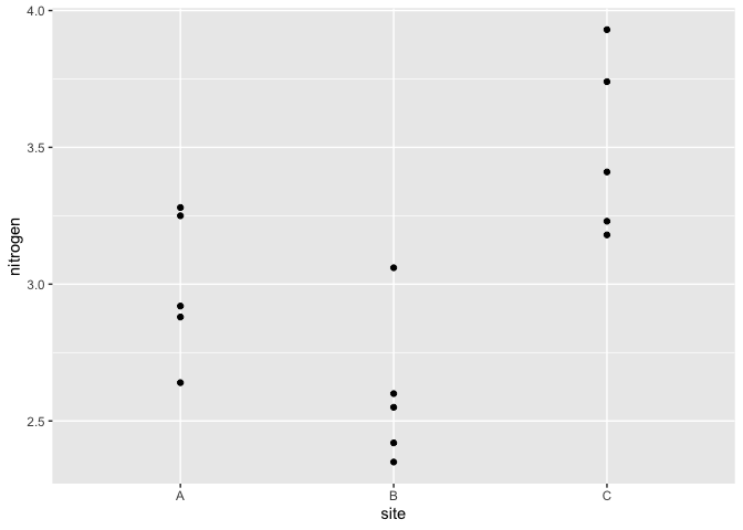
Plot the data which shows the nitrogen content of samples of reeds at three different sites. The specific sites themselves are not important but we are interested in how the response might vary between sites.
ggplot(reeds,aes(site,nitrogen))+geom_point()
Standard MLE analysis
We can fit a model with a fixed effect for the intercept and a random
effect for the site using lme4:
library(lme4)
mmod <- lmer(nitrogen ~ 1+(1|site), reeds)
summary(mmod)
Linear mixed model fit by REML ['lmerMod']
Formula: nitrogen ~ 1 + (1 | site)
   Data: reeds

REML criterion at convergence: 13

Scaled residuals:
   Min     1Q Median     3Q    Max
-1.221 -0.754 -0.263  0.914  1.612

Random effects:
 Groups   Name        Variance Std.Dev.
 site     (Intercept) 0.1872   0.433
 Residual             0.0855   0.292
Number of obs: 15, groups:  site, 3

Fixed effects:
            Estimate Std. Error t value
(Intercept)    3.029      0.261    11.6
These are REML rather than ML estimates to be precise
Default INLA
Now try INLA:
formula <- nitrogen ~ 1 + f(site, model="iid")
imod  <-  inla(formula,family="gaussian", data = reeds)
We can get the fixed effect part of the output from:
imod$summary.fixed
              mean      sd 0.025quant 0.5quant 0.975quant   mode       kld
(Intercept) 3.0293 0.13496     2.7644   3.0293      3.294 3.0293 0.0022404
which is quite similar to the REML result. The random effect summary can be extracted with:
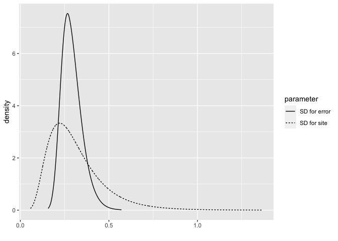
bri.hyperpar.summary(imod)
                                    mean      sd  q0.025    q0.5  q0.975    mode
SD for the Gaussian observations 0.29079 0.05833 0.19817 0.28283 0.42608 0.26647
SD for site                      0.31313 0.15740 0.10893 0.27910 0.71369 0.22176
We can plot the posterior densities of the random effects with:
bri.hyperpar.plot(imod)
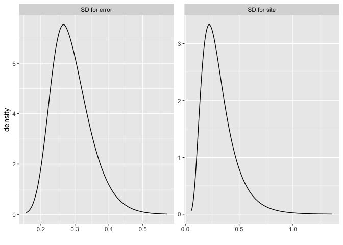
or separately as:
bri.hyperpar.plot(imod, together=FALSE)
y=Xb+Zu+e model
Mixed effects models are sometimes presented in a y=Xb+Zu+e form where
X is the design matrix of the fixed effects and Z is the design
matrix of the random effects. The lme4 package makes it easy to
extract the X and Z:
Z = getME(mmod, "Z")
X = getME(mmod, "X")
We can the use INLA to fit the model in this form. Note the -1 is
because X already has an intercept column.
n = nrow(reeds)
formula = y ~ -1 + X +  f(id.z, model="z",  Z=Z)
imodZ = inla(formula, data = list(y=reeds$nitrogen, id.z = 1:n, X=X))
We can get the fixed effects as:
imodZ$summary.fixed
              mean      sd 0.025quant 0.5quant 0.975quant   mode       kld
(Intercept) 3.0293 0.13496     2.7644   3.0293      3.294 3.0293 0.0022396
and the random effects in terms of the SDs as
bri.hyperpar.summary(imodZ)
                                    mean      sd  q0.025    q0.5  q0.975    mode
SD for the Gaussian observations 0.29079 0.05833 0.19817 0.28283 0.42608 0.26647
SD for id.z                      0.31313 0.15740 0.10893 0.27909 0.71371 0.22176
which is identical to the previous result. Although the two methods are equivalent here, we will probably find it easier to get the information we need from the first approach when we have more complex random effects.
Penalized Complexity Prior
In Simpson et al (2015), penalized complexity priors are proposed. This requires that we specify a scaling for the SDs of the random effects. We use the SD of the residuals of the fixed effects only model (what might be called the base model in the paper) to provide this scaling.
sdres <- sd(reeds$nitrogen)
pcprior <- list(prec = list(prior="pc.prec", param = c(3*sdres,0.01)))
formula <- nitrogen ~ f(site, model="iid", hyper = pcprior)
imod <- inla(formula, family="gaussian", data=reeds)
Fixed effects
imod$summary.fixed
              mean      sd 0.025quant 0.5quant 0.975quant   mode        kld
(Intercept) 3.0293 0.30497      2.404   3.0293      3.655 3.0293 0.00025399
random effects
bri.hyperpar.summary(imod)
                                    mean       sd  q0.025    q0.5  q0.975    mode
SD for the Gaussian observations 0.28651 0.055529 0.19794 0.27906 0.41494 0.26358
SD for site                      0.46599 0.219838 0.18247 0.41706 1.02813 0.33867
which can be plotted as:
bri.hyperpar.plot(imod)
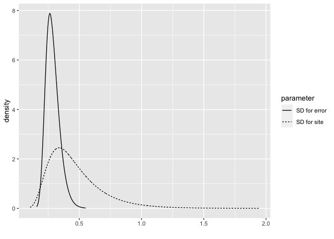
This results in a larger posterior for the site SD. Hence the PC prior is putting more weight on larger SDs.
Random effects
We can plot the random effect posterior densities for the three sites:
reff <- imod$marginals.random
x <- seq(-1.5,1.5,len=100)
d1 <- inla.dmarginal(x, reff$site[[1]])
d2 <- inla.dmarginal(x, reff$site[[2]])
d3 <- inla.dmarginal(x, reff$site[[3]])
rdf <- data.frame(bright=c(x,x,x),density=c(d1,d2,d3),site=gl(3,100,labels=LETTERS[1:3]))
ggplot(rdf, aes(x=bright, y=density, color=site))+geom_line()
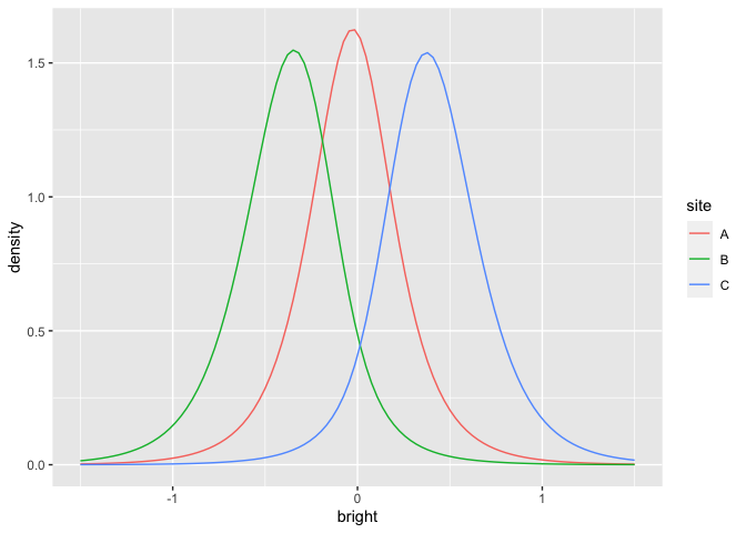
What is the probability that a sample from site B would exceed the nitrogen in a sample from site C? We can answer this question with a sample from the posterior:
imod <- inla(formula, family="gaussian", data=reeds, control.compute=list(config = TRUE))
psamp = inla.posterior.sample(n=1000, imod)
lvsamp = t(sapply(psamp, function(x) x$latent))
colnames(lvsamp) = make.names(row.names(psamp[[1]]$latent))
plot(site.2 ~ site.3, lvsamp)
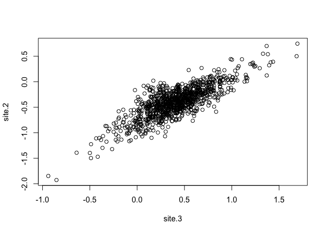
mean(lvsamp[,'site.2'] > lvsamp[,'site.3'])
[1] 0
Although the site posteriors overlap in the figure, the positive correlation between the two variables means that the chance of B>C is negligible.