brinla
Non-stationary smoothing with Gaussian process regression using INLA
Julian Faraway 21 September 2020
See the introduction for more about INLA. See an example of Gaussian process regression. The construction is detailed in our book.
Load the packages (you may need to install the brinla package)
library(INLA)
library(brinla)
Data
We simulate some data with a known true function.
set.seed(1)
n <- 100
x <- seq(0, 1, length = n)
f.true <- (sin(2 * pi * (x)^3))^3
y <- f.true + rnorm(n, sd = 0.2)
td <- data.frame(y = y, x = x, f.true)
and plot it:
plot(y ~ x, td)
lines(f.true ~ x, td)
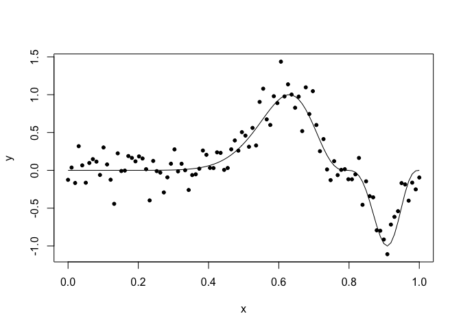
This function is challenging to fit because of the varying amount of smoothness. You can see examples of various smoothing methods applied to this data in (Faraway 2016).
GP fitting
The default fit uses priors based on the SD of the response and the range of the predictor to motivate sensible priors.
gpmod = bri.gpr(td$x, td$y)
We can plot the resulting fit and 95% credible bands
plot(y ~ x, td, col = gray(0.75))
lines(gpmod$xout, gpmod$mean)
lines(gpmod$xout, gpmod$lcb, lty=2)
lines(gpmod$xout, gpmod$ucb, lty=2)
lines(f.true ~ x, td, col=2)
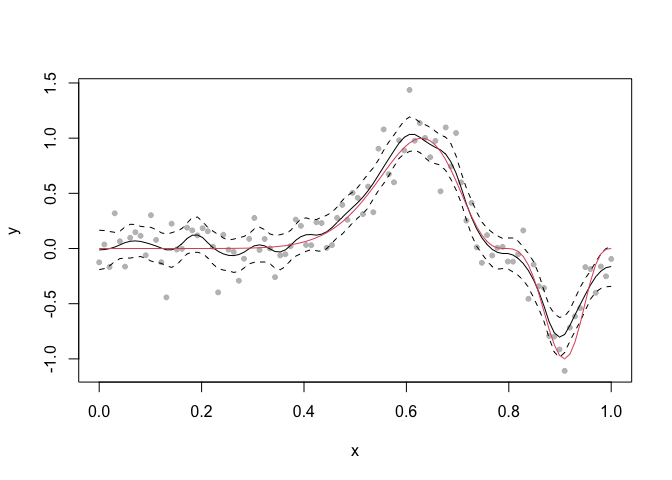
On the right end of the function, the fit is too rough. On the left end, it is too smooth. The minimum at 0.9 is underestimated and the true function is even outside the credibility bands in this region. The problem is that the standard method uses the same amount of smoothness everywhere.
Variable smoothness
We can allow the smoothness to vary. A description of this can be found
in (Lindgren and Rue 2015) and also in our
book. We have implemented this
in our brinla package:
fg <- bri.nonstat(td$x, td$y)
plot(y ~ x, td, col = gray(0.75))
lines(f.true ~ x, td, col = 2)
lines(fg$xout, fg$lcb, lty=2)
lines(fg$xout, fg$ucb, lty=2)
lines(fg$xout, fg$mean)
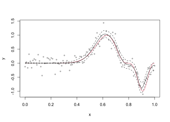
We achieve a smoother fit on the left but keep the less smooth fit on the right.
Package versions
sessionInfo()
R version 4.0.2 (2020-06-22)
Platform: x86_64-apple-darwin17.0 (64-bit)
Running under: macOS Catalina 10.15.6

Matrix products: default
BLAS:   /Library/Frameworks/R.framework/Versions/4.0/Resources/lib/libRblas.dylib
LAPACK: /Library/Frameworks/R.framework/Versions/4.0/Resources/lib/libRlapack.dylib

locale:
[1] en_GB.UTF-8/en_GB.UTF-8/en_GB.UTF-8/C/en_GB.UTF-8/en_GB.UTF-8

attached base packages:
[1] parallel  stats     graphics  grDevices utils     datasets  methods   base

other attached packages:
[1] brinla_0.1.0  INLA_20.03.17 foreach_1.5.0 sp_1.4-2      Matrix_1.2-18 knitr_1.29

loaded via a namespace (and not attached):
 [1] codetools_0.2-16     lattice_0.20-41      digest_0.6.25        grid_4.0.2           MatrixModels_0.4-1
 [6] magrittr_1.5         evaluate_0.14        rlang_0.4.7          stringi_1.4.6        rmarkdown_2.3
[11] splines_4.0.2        iterators_1.0.12     tools_4.0.2          stringr_1.4.0        xfun_0.16
[16] yaml_2.2.1           compiler_4.0.2       htmltools_0.5.0.9000