brinla
INLA for linear regression
Julian Faraway 21 September 2020
In this example, we compare the Bayesian model output with the linear model fit. Although the interpretation of these two fits is different, we expect similar numerical results provided the priors are not informative.
See the introduction for an overview. Load the packages: (you may need to install them first)
library(ggplot2)
library(INLA)
Loading required package: Matrix

Loading required package: sp

Loading required package: parallel

Loading required package: foreach

This is INLA_20.03.17 built 2020-09-21 11:41:39 UTC.
See www.r-inla.org/contact-us for how to get help.
To enable PARDISO sparse library; see inla.pardiso()
library(faraway)
library(gridExtra)
library(brinla)
Data
Load in the Chicago Insurance dataset as analyzed in Linear Models with R:
data(chredlin, package="faraway")
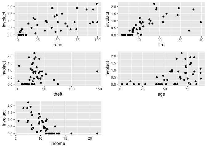
We take involact as the response. Make some plots of the data:
p1=ggplot(chredlin,aes(race,involact)) + geom_point()
p2=ggplot(chredlin,aes(fire,involact)) + geom_point()
p3=ggplot(chredlin,aes(theft,involact)) + geom_point()
p4=ggplot(chredlin,aes(age,involact)) + geom_point()
p5=ggplot(chredlin,aes(income,involact)) + geom_point()
grid.arrange(p1,p2,p3,p4,p5)
Linear model analysis
Fit the standard linear model for reference purposes:
lmod <- lm(involact ~ race + fire + theft + age + log(income),  chredlin)
sumary(lmod)
            Estimate Std. Error t value Pr(>|t|)
(Intercept) -1.18554    1.10025   -1.08  0.28755
race         0.00950    0.00249    3.82  0.00045
fire         0.03986    0.00877    4.55  4.8e-05
theft       -0.01029    0.00282   -3.65  0.00073
age          0.00834    0.00274    3.04  0.00413
log(income)  0.34576    0.40012    0.86  0.39254

n = 47, p = 6, Residual SE = 0.335, R-Squared = 0.75
INLA default model
Run the default INLA model and compare to the lm output:
formula <- involact ~ race + fire + theft + age + log(income)
imod <- inla(formula, family="gaussian", data=chredlin)
cbind(imod$summary.fixed[,1:2],summary(lmod)$coef[,1:2])
                  mean        sd   Estimate Std. Error
(Intercept) -1.1853891 1.0979085 -1.1855396  1.1002549
race         0.0095020 0.0024844  0.0095022  0.0024896
fire         0.0398555 0.0087480  0.0398560  0.0087661
theft       -0.0102944 0.0028121 -0.0102945  0.0028179
age          0.0083354 0.0027383  0.0083356  0.0027440
log(income)  0.3457063 0.3992695  0.3457615  0.4001234
The first two columns are the posterior means and SDs from the INLA fit while the third and fourth are the corresponding values from the lm fit. We can see they are almost identical. We expect this.
We can get the posterior for the SD of the error as:
bri.hyperpar.summary(imod)
                                    mean       sd  q0.025    q0.5  q0.975    mode
SD for the Gaussian observations 0.33244 0.036546 0.27005 0.32914 0.41338 0.32274
which compares with the linear model estimate of:
summary(lmod)$sigma
[1] 0.33453
which gives a very similar result. But notice that the Bayesian output gives us more than just a point estimate.
The function inla.hyperpar() is advertized to improve the estimates of
the hyperparameters (just sigma here) but makes very little difference
in this example:
bri.hyperpar.summary(inla.hyperpar(imod))
                                    mean       sd  q0.025    q0.5 q0.975    mode
SD for the Gaussian observations 0.33245 0.036554 0.27005 0.32914 0.4134 0.32274
Plots of the posteriors
For the error SD
bri.hyperpar.plot(imod)
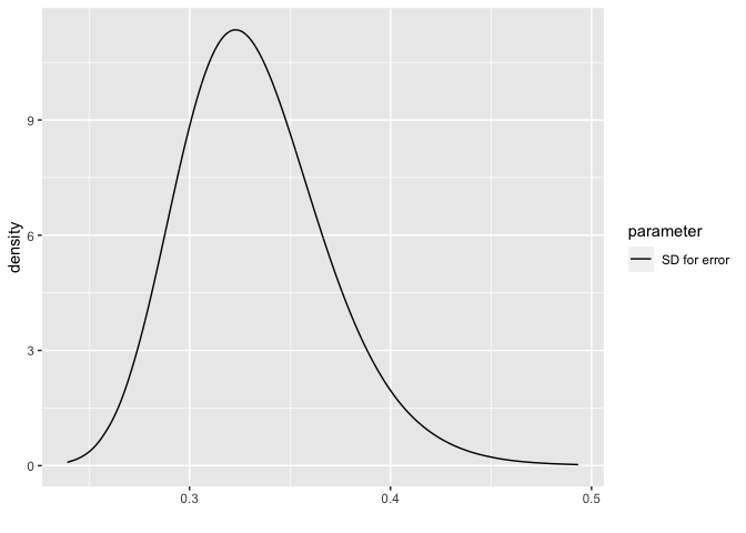
For the fixed parameters:
bri.fixed.plot(imod)
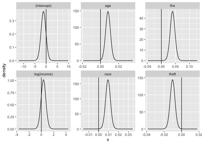
We can use these plots to judge which parameters may be different from zero. For age, fire, race and theft, we see the posterior density is well away from zero but for log(income) there is an overlap. This can be qualitatively compared to the p-values from the linear model output. The conclusions are compatible although the motivation and justifactions are different.
Fitted values
We need to set the control.predictor to compute the posterior means of the linear predictors:
result <- inla(formula, family="gaussian", control.predictor=list(compute=TRUE),data=chredlin)
ypostmean <- result$summary.linear.predictor
Compare these posterior means to the lm() fitted values:
plot(ypostmean[,1],lmod$fit, xlab="INLA posterior fitted means", ylab="LM fitted values")
abline(0,1)
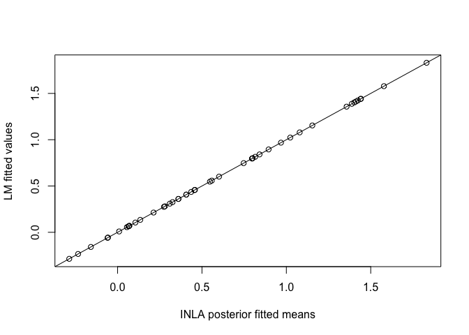
Can see these are the same. Now compare the SDs from INLA with the SEs from the LM fit:
lmfit <- predict(lmod, se=TRUE)
plot(ypostmean[,2], lmfit$se.fit, xlab="INLA posterior SDs", ylab="LM fitted SEs")
abline(0,1)
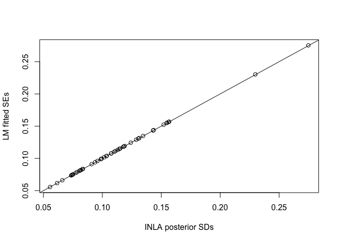
We see that these are the same.
Prediction
Suppose we wish to predict the response at a new set of inputs. We add a case for the new inputs and set the response to missing:
newobs = data.frame(race=25,fire=10,theft=30,age=65,involact=NA,income=11,side="s")
chpred = rbind(chredlin,newobs)
We fit the model as before:
respred <- inla(formula, family="gaussian", control.predictor=list(compute=TRUE), data=chpred)
respred$summary.fixed
                  mean        sd 0.025quant   0.5quant 0.975quant       mode        kld
(Intercept) -1.1853891 1.0979084 -3.3512580 -1.1854262  0.9787808 -1.1853992 2.5514e-05
race         0.0095020 0.0024844  0.0046010  0.0095019  0.0143991  0.0095020 2.5522e-05
fire         0.0398555 0.0087480  0.0225979  0.0398553  0.0570993  0.0398556 2.5526e-05
theft       -0.0102944 0.0028121 -0.0158419 -0.0102945 -0.0047513 -0.0102944 2.5527e-05
age          0.0083354 0.0027383  0.0029334  0.0083353  0.0137331  0.0083354 2.5525e-05
log(income)  0.3457063 0.3992695 -0.4419491  0.3456954  1.1327297  0.3457100 2.5513e-05
The output is the same as before as expected. The fitted value for the last observation (the new 48th observation) provides the posterior distribution for the linear predictor corresponding to the new set of inputs.
respred$summary.fitted.values[48,]
                       mean       sd 0.025quant 0.5quant 0.975quant    mode
fitted.Predictor.48 0.51265 0.054281     0.4057  0.51265     0.6196 0.51265
We might compare this to the standard linear model prediction:
predict(lmod, newdata=newobs, interval = "confidence", se=TRUE)
$fit
      fit     lwr     upr
1 0.51266 0.40292 0.62239

$se.fit
[1] 0.054337

$df
[1] 41

$residual.scale
[1] 0.33453
We get the essentially the same outcome. These answers only reflect variability in the linear predictor.
Usually we want to include the variation due to a new error. This requires more effort. One solution is based on simulation. We can sample from the posterior we have just calculated and sample from the posterior for the error distribution. Adding these together, we will get a sample from the posterior predictive distribution. Although this can be done quickly, it goes against the spirit of INLA by using simulation.
We can compute an approximation for the posterior predictive
distribution using some trickery. We set up an index variable idx. We
add a random effect term using this index with the f() function.
This is a mean zero Gaussian random variable whose variance is a
hyperparameter. This term functions exactly the same as the usual error
term. Since the model will also add an error term, we would be stuck
with two essentially identical terms. But we are able to knock out the
usual error term by specifying that it have a very high precision
(i.e. it will vary just a little bit). In this way, our random effect
term will take almost all the burden of representing this variation.
chpred$idx <- 1:48
eformula <- involact ~ race + fire + theft + age + log(income) + f(idx, model="iid", hyper = list(prec = list(param=c(1, 0.01))))
respred <- inla(eformula, data = chpred, control.predictor = list(compute=TRUE), control.family=list(initial=12,fixed=TRUE))
bri.hyperpar.summary(respred)
              mean       sd  q0.025    q0.5  q0.975    mode
SD for idx 0.33315 0.036626 0.27063 0.32984 0.41427 0.32342
We see that the SD for the index variable is about the same as the previous SD for the error. Look at the predictive distribution:
respred$summary.fitted.values[48,]
                       mean      sd 0.025quant 0.5quant 0.975quant    mode
fitted.Predictor.48 0.51266 0.33893   -0.15516  0.51265     1.1804 0.51265
We can compare this to the linear model prediction interval:
predict(lmod,newdata=newobs,interval="prediction")
      fit      lwr    upr
1 0.51266 -0.17179 1.1971
The results are similar but not the same. Notice that the lower end of the intervals are both negative which should not happen with a strictly positive response. But that’s not the fault of this process but of our choice of model.
Here is a posterior predictive density for the prediction:
ggplot(data.frame(respred$marginals.fitted.values[[48]]),aes(x,y))+geom_line()+ylab("Density")+xlab("involact")
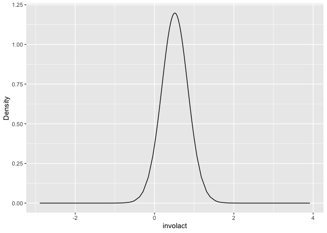
We see the problem of having density for values less than zero.
For more on this, see the Google groups INLA mailing list discussion.
Conditional Predictive Ordinates and Probability Integral Transform
Bayesian diagnostic methods can use these statistics. We need to ask for them at the time we fit the model:
imod <- inla(formula, family="gaussian", data=chredlin, control.compute=list(cpo=TRUE))
The CPO is the probability density of an observed response based on the model fit to the rest of the data. We are interested in small values of the CPO since these represent unexpected response values. Plot the CPOs:
n = nrow(chredlin)
plot(1:n,imod$cpo$cpo, ylab="CPO",type="n")
text(1:n,imod$cpo$cpo, 1:n)
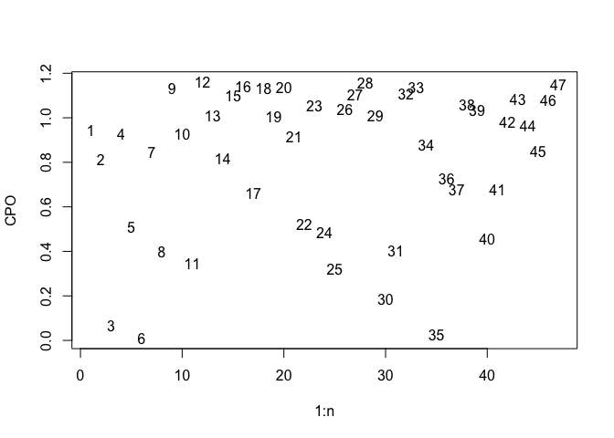
Observations 3, 6 and 35 have particularly low values. We might compare these to the jacknife residuals (an analogous quantity) from the standard linear model:
plot(imod$cpo$cpo, abs(rstudent(lmod)), xlab="CPO",ylab="Absolute residuals", type="n")
text(imod$cpo$cpo, abs(rstudent(lmod)), 1:n)
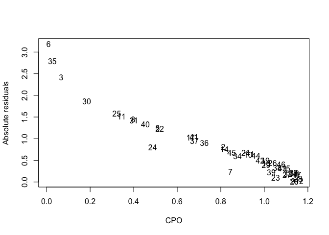
We can see the two statistics are related. They pick out the same three observations.
The PIT is the probability of a new response less than the observed response using a model based on the rest of the data. We’d expect the PIT values to be uniformly distributed if the model assumptions are correct.
pit <- imod$cpo$pit
uniquant <- (1:n)/(n+1)
plot(uniquant, sort(pit), xlab="uniform quantiles", ylab="Sorted PIT values")
abline(0,1)
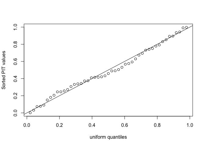
Looks good - no indication of problems. Might be better to plot these on a logit scale because probabilities very close to 0 or 1 won’t be obvious from the above plot.
plot(logit(uniquant), logit(sort(pit)), xlab="uniform quantiles", ylab="Sorted PIT values", main="Logit scale")
abline(0,1)
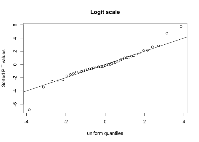
This marks out three points as being somewhat unusual:
which(abs(logit(pit)) > 4)
[1] 3 6 35
The same three points picked out by the CPO statistic.
We can compare the PIT values and posterior means for the fitted values (which are the same as the fitted values from the linear model fit).
plot(predict(lmod), pit, xlab="Posterior fitted means", ylab="PIT")
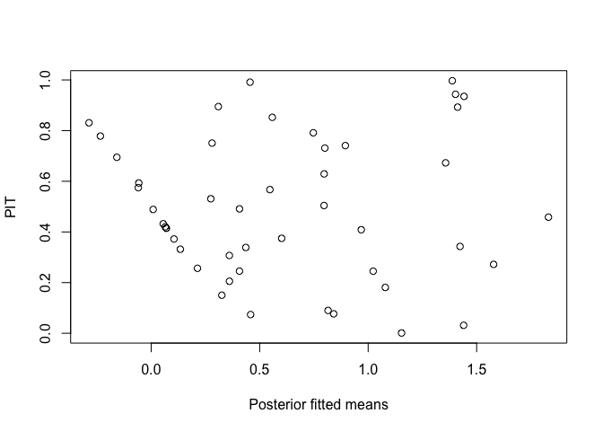
This indicates some problems for low values. Since the response is strictly positive and this is not reflected in our models, this does spot a real flaw in our model.
Incidentally, a similar conclusion can be made from the standard linear model diagnostic:
plot(lmod,1)
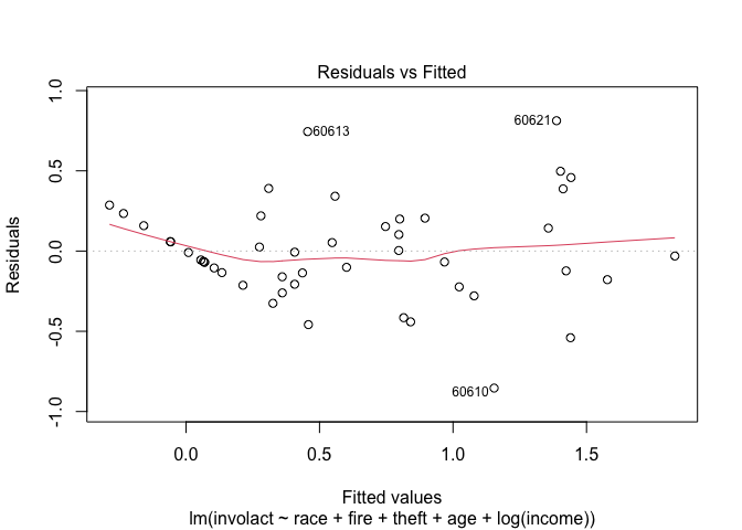
which looks fairly similar. In this example, we might try something other than a Gaussian response which reflects the zero response values.
We can also plot the PITs against the predictors - for example:
plot(chredlin$race, pit, xlab="Minority percentage", ylab="PIT")
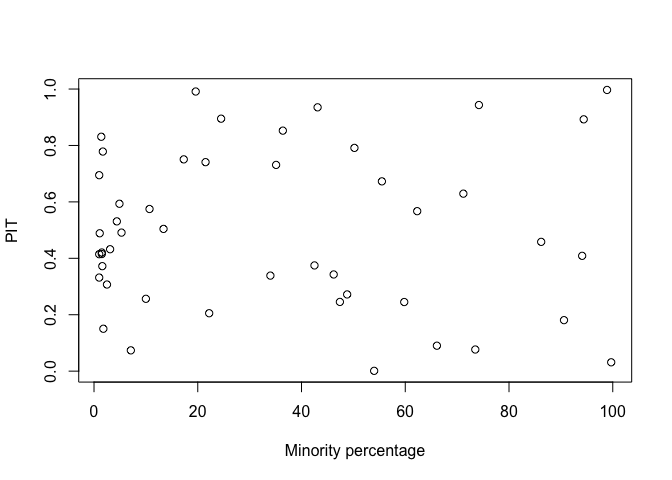
Which shows no problems with the fit.
Model Selection
We need to ask to get the Watanabe AIC (WAIC) and deviance information criterion DIC calculated:
imod <- inla(formula, family="gaussian", data=chredlin, control.compute=list(dic=TRUE, waic=TRUE))
which produces:
c(WAIC=imod$waic$waic, DIC=imod$dic$dic)
  WAIC    DIC
40.151 38.611
We do not have many predictors here so exhaustive search is feasible. We
fit all models that include race but with some combination of the other
four predictors. Use lm() to get the AIC but INLA to get DIC and WAIC
listcombo <- unlist(sapply(0:4,function(x) combn(4, x, simplify=FALSE)),recursive=FALSE)
predterms <- lapply(listcombo, function(x) paste(c("race",c("fire","theft","age","log(income)")[x]),collapse="+"))
coefm <- matrix(NA,16,3)
for(i in 1:16){
    formula <- as.formula(paste("involact ~ ",predterms[[i]]))
    lmi <- lm(formula, data=chredlin)
    result <- inla(formula, family="gaussian", data=chredlin, control.compute=list(dic=TRUE, waic=TRUE))
    coefm[i,1] <- AIC(lmi)
    coefm[i,2] <- result$dic$dic
    coefm[i,3] <- result$waic$waic
}
rownames(coefm) <- predterms
colnames(coefm) <- c("AIC","DIC","WAIC")
round(coefm,4)
                                   AIC    DIC   WAIC
race                            62.032 62.216 62.416
race+fire                       50.744 50.990 54.014
race+theft                      63.925 64.171 64.073
race+age                        54.026 54.273 54.304
race+log(income)                57.883 58.129 58.572
race+fire+theft                 43.970 44.303 46.623
race+fire+age                   47.306 47.639 50.031
race+fire+log(income)           51.412 51.744 54.445
race+theft+age                  54.252 54.585 54.597
race+theft+log(income)          59.591 59.923 60.360
race+age+log(income)            54.804 55.137 55.152
race+fire+theft+age             36.876 37.321 39.117
race+fire+theft+log(income)     45.569 46.013 48.202
race+fire+age+log(income)       49.272 49.717 51.793
race+theft+age+log(income)      55.215 55.660 55.810
race+fire+theft+age+log(income) 38.028 38.611 40.151
The model corresponding to the minimum value of the criterion is the
same for all three. We would choose involact ~ race+fire+theft+age.
Conclusion
We see that the standard linear modeling and the Bayesian approach using INLA produce very similar results. On one hand, one might decide to stick with the standard approach since it is easier. But on the other hand, this does give the user confidence to use the Bayesian approach with INLA because it opens up other possibilities with the model fitting and interpretation. The consistency between the approaches in the default settings is reassuring.